Brain Atrophy - Processing Options for Cross-Sectional Assessment

Brain Atrophy - Cross-Sectional

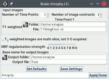
The picture below shows the setup for assessing brain atrophy at a single time-point (cross-sectionally) using just a T₁-weighted image.

Setup for cross-sectional brain atrophy assessment

The input image should, ideally, have been acquired using a 3-D (not multi-slice) pulse sequence. Follow these steps for cross-sectional atrophy assessment:

Load the T₁-weighted image in the input image selection panel. In the example above, this is called "T1Weighted.nii".
. If the T₁-weighted image was acquired multi-slice (with slice selection), rather than 3-D (with the slice dimension being phase-encoded), then select this option.
Leave the slider at its default value of 5. This should not need to be changed.
Set the base name and folder for the output images.
Optional. If you want to use a FLAIR image as well, increase the number of contrasts to 2, and select the FLAIR image.

Now press the Button to start the atrophy analysis

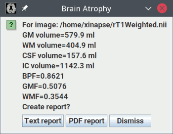
button to start the analysis, which will take some time. When the analysis is complete, you will see a pop-up message showing the results:

Results for cross-sectional brain atrophy assessment

These results show:

The grey-matter (GM) volume.
The white-matter (WM) volume.
The cerebro-spinal fluid (CSF) volume.
The intra-cranial volume (ICV), which is the sum of the volumes of the 3 compartments above.
The brain parenchymal fraction (BPF), which is: (GM Volume + WM Volume) / ICV.
The grey-matter fraction (GMF), which is: GM Volume / ICV.
The white-matter fraction (WMF), which is: WM Volume / ICV.

To make a permanent record of these results, you can:

Write to a text file report. A File chooser will appear, for you to choose a log file name. The default file extension for log files is ".log". If the chosen file already exists, an entry will be appended to the log file.
Write to a PDF file report. A File chooser will appear, for you to choose a PDF file name. If the chosen file already exists, an entry will be appended to the PDF file. A PDF report will also include an illustration the GM/WM/CSF segmentation.

For an input image called "T1Weighted.nii" and a base name of "Test", these output images will be created in the selected folder:

TestGMPrior.nii - the grey-matter prior probability image, registered to the T₁-weighted image.
TestWMPrior.nii - the white-matter prior probability image, registered to the T₁-weighted image.
TestCSFPrior.nii - the CSF prior probability image, registered to the T₁-weighted image.
TestLVPrior.nii - the lateral ventricles prior probability image, registered to the T₁-weighted image.
TestPosition.nii - an image of the pixel positions in template image space.
rT1Weighted_pGM.nii - the grey-matter posterior probability image.
rT1Weighted_pWM.nii - the white-matter posterior probability image.
rT1Weighted_pCSF.nii - the CSF posterior probability image.
rT1Weighted_pOTHER.nii - the other (non-tissue) class posterior probability image.
rT1Weighted_Classes.nii - a colour image showing the final segmented tissue classes.

rT1Weighted.nii - a cropped version of the T₁-weighted input image and bcrT1Weighted.nii, a bias-corrected version of this.

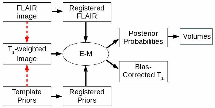
The procedure for cross-sectional atrophy assessment is summarised in the flow-chart below.

The flow chart for cross-sectional brain atrophy assessment

The red arrows indicate a registration step, with the arrow pointing towards the registration target. The use of the FLAIR image is optional. E-M: expectation-maximization classification algorithm.

Jim Home