Dynamic Analysis - Roaming Intensities

Once you have set up the Dynamic Analysis tool to perform the analysis as required, you can:

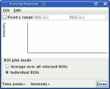
Click on the image to view the time series of pixel intensities at the mouse location, or
View the time series of pixel intensities inside a region of interest. The intensity values shown are the mean pixel intensities within the ROI, for each time point.

The intensities are viewed on a pop-up graph.

First, set up the input images, as described in the Introduction. Next, load an image into Jim. The image you load can be any of the input images (or the input image if you have just a single input image).

To view the time series of intensities, select Roam ... from the View menu of the tool: dynamic_view_roam . Both the ROI Toolkit, and the Roaming Response dialog will pop up.

dynamic_roaming_response_dialog

Then, either:

Click on the image with the mouse. The intensities for each time point will be extracted from the image(s) at the mouse position.
Using the ROI Toolkit, create a region of interest on the image you are viewing in Jim. The mean intensity values will be extracted from the input images within the ROI you just created. If you select more than one ROI, depending on the selection:

you will plot either:
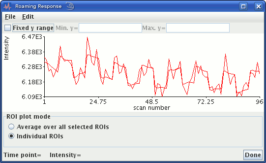
- The average intensity averaged over all the selected ROIs, or
- The signal intensity from each ROI individually. In this mode, the colour of the line for each will match the colour of the ROI, allowing you identify which line belongs to which ROI by changing the ROI's colour.

The time-series will be displayed in the Roaming Response dialog, and if your have correctly setup a model, such as the General Linear Model, the model fit to the data will also be shown, as in the plot below.

glm_plot_dialog
Signal intensity and fitted general linear model fit in an area of activation in an fMRI experiment.

Note: the graph may take a long time to appear (several seconds), since all the input images must be opened and the pixel intensity values read before the graph can be computed. Whenever you load new input image(s) into the tool, there will be a delay before the graph can be updated, since these new images must also be opened.

You can drag the ROIs around the image, or create other ROIs and see how the time course of pixel intensities varies across the image.

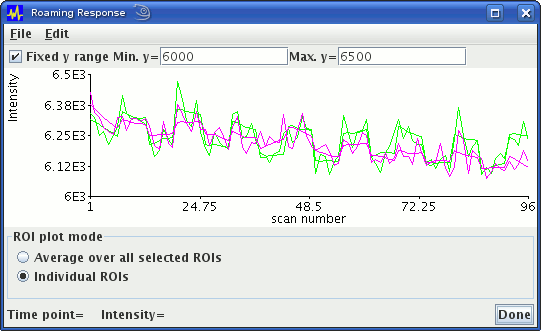
The y (intensity) data ranges of the graph are automatically scaled to match the data. If you want to fix the range of data on the y-axis, select the "Fixed y range" check box, and type in a range that you want to be displayed. Note: If you make changes to the setup in the model, the graph may not be be updated until you de-select and re-select the ROI.

glm_plot_dialog_2_regions
Signal intensity and fitted general linear model in two areas of activation in an fMRI experiment, with a fixed intensity range.

You can write the graph data to a disk file by selecting Write from the File menu: file_write

The graph data is written in a tab-separated table with two columns: the first is the scan number value and the second is the pixel intensity. See also the File Formats section.

To create a screen shot of the graph, select Create a screen shot of a graph , then, in the next dialog, select the image file format you want.

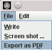
You can write the graph to a PDF document by selecting Export as PDF from the File menu: file_export_pdf

Jim Home