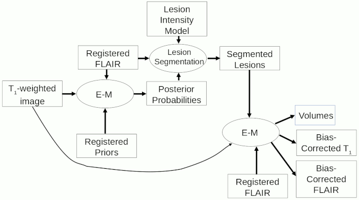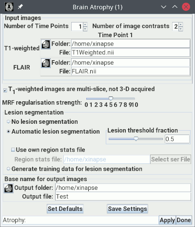
The picture below shows the setup for assessing brain atrophy at a single time-point (cross-sectionally) when there are white-matter (WM) lesions present. For this, you need both a T1-weighted image and a FLAIR image.
T1Weighted.nii".
Load the FLAIR image in the second input image
selection panel. In the example above, this is called "FLAIR.nii".
 .
If the T1-weighted image was acquired multi-slice (with slice
selection), rather than 3-D (with the slice dimension being
phase-encoded), then select this option.
.
If the T1-weighted image was acquired multi-slice (with slice
selection), rather than 3-D (with the slice dimension being
phase-encoded), then select this option.
 slider at its
default value of 5. This should not need to be changed.
slider at its
default value of 5. This should not need to be changed.
 . Jim
has been trained to segment WM lesions using a selection of images
from different MR scanners with variations in pulse
sequence. However, if your images have unusual contrast (particularly
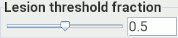
the FLAIR images) then you may need to change the "lesion threshold
fraction" setting from its default value of 0.5.
Either move the slider, or type in a value between 0 and 1.
. Jim
has been trained to segment WM lesions using a selection of images
from different MR scanners with variations in pulse
sequence. However, if your images have unusual contrast (particularly
the FLAIR images) then you may need to change the "lesion threshold
fraction" setting from its default value of 0.5.
Either move the slider, or type in a value between 0 and 1.
If you trained the lesion
segmentation using your own data, you will need to select
 ,
and set the file containing the trained image region statistics using:
,
and set the file containing the trained image region statistics using:
 .
.
 button to
start the analysis, which will take some time.
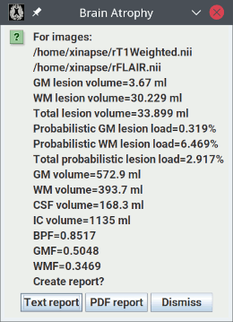
When the analysis is complete, you will see a pop-up message showing the results:
button to
start the analysis, which will take some time.
When the analysis is complete, you will see a pop-up message showing the results:
TestGMPrior.nii - the grey-matter prior probability image, registered to
the cropped T1-weighted image.TestWMPrior.nii - the white-matter prior probability image, registered to
the cropped T1-weighted image.TestCSFPrior.nii - the CSF prior probability image, registered to
the cropped T1-weighted image.TestLVPrior.nii - the lateral ventricles prior
probability image, registered to the cropped T1-weighted image.TestPosition.nii - an image of the pixel positions in
template image space.
rT1Weighted_pGM.nii - the grey-matter posterior
probability image.rT1Weighted_pWM.nii - the white-matter posterior
probability image.rT1Weighted_pCSF.nii - the CSF posterior probability
image.rT1Weighted_pOTHER.nii - the other (non-tissue)
class posterior probability image.rT1Weighted_Classes.nii - a colour image showing the
final segmented tissue classes.
rT1Weighted.nii - a cropped version of the T1-weighted
input image and bcrT1Weighted.nii, a bias-corrected version of this.rFLAIR.nii - the FLAIR image registered to
the cropped T1-weighted image
and bcrFLAIR.nii, a bias-corrected version of
this."rFLAIR.roi", where the
ROIs outline the segmented lesions on every image slice. These ROIs can
be reviewed by
loading
them onto either rFLAIR.nii or bcrFLAIR.nii, to ensure that the outlining of lesions is
satisfactory. If the outlining is not satisfactory, you can either:
Note: if you do not delete the lesion ROI file, Jim will not re-segment the lesions, and the change in threshold will have no effect.
Note: when the analysis is repeated like this, as long as the output images initally produced are not removed, and the output images Basename is not changed, then the analysis will run in a much shorter time, since intermediate registration steps can be skipped.
The procedure for cross-sectional atrophy assessment when hyperintense lesions are present (after the registration steps), is summarised in the flow-chart below.