Dynamic Analysis - General Linear Model

The General Linear Model module performs a GLM analysis of the time-series of input images, and is capable of sophisticated analysis of (amongst other things) fMRI data and arterial spin labelling perfusion data. The GLM assumes that the signal changes you see in the time-series consists of linear combination of a set of 'basis' functions. The GLM estimates the amplitudes (weights) of the basis functions such that when they are added together, they form a least-squares fit to the time-series.

You can choose the General Linear Model module by clicking the tab in the Dynamic Analysis tool.

dynamic_glm

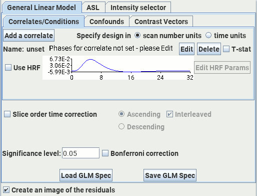
The General Linear Model tab contains three of its own tabs: "Correlates/Conditions", "Confounds" and "Contrast Vectors". These are described below.

Correlates/Conditions

A correlate (or condition) forms a single basis function to be fitted to the time-series. You can build up a model of your data using as many correlates as you need to model your data. For example, in fMRI experiments, each independent 'task' would contribute one basis function. If you have multiple simultaneous tasks going on, use a correlate for each one. Add as many correlates as you need to describe the data by pressing the add_correlate_button

button. To delete a correlate, click on the delete_button

button for that correlate.

Before creating correlates, decide whether you want to construct your correlates as functions of time or scan number. Select either:

times of onset etc. will be specified with respect to the scan number; or
times of onset etc. will be specified in seconds from the start of the scanning.

For each correlate that you have, you will need to construct the basis function for that correlate. To construct the basis function, click the edit_button button. This will bring up a dialog asking how you want to construct the correlate:

glm_correlate_design

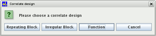
Select one of:

if the thing you are correlating to repeats in a regular on-off pattern, such as in a regular block-design fMRI experiment. Selecting "Repeating Block" brings up the repeating block design dialog:

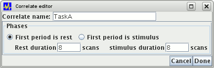
You need to:
1. Give your correlate a name (in the "Correlate name" field), such as "TaskA".
2. Set whether the first phase of your task is a resting period () or a period of stimulus ().
3. Set the duration of the rest periods and the duration of the stimulus periods. For a repeating block correlate, all rest periods must be the same duration and all stimulus periods must be the same duration. Enter the durations either in seconds or in scan units, depending on the setting or .
Above, we have set a correlate called "TaskA" that repeats every 16 scans, with the same time interval for rest and stimulus (8 scans each).
Click the button when you are finished, and a sketch of the design matrix will be shown in the General Linear Model tab for the correlate you just created.
if the thing you are correlating to repeats in a irregular on-off pattern, such as in an irregular block-design fMRI experiment. Selecting "Irregular Block" brings up the irregular block design dialog:

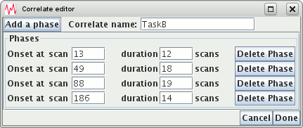
An irregular block design consists of a number (1 or more) phases. One phase consists of a period or rest, followed by a period of stimulus, followed by a period of rest. You can have as many phases are you need, but the phases for one irregular block correlate may not overlap. You need to:
1. Give your correlate a name (in the "Correlate name" field), such as "TaskA".
2. Add as many phases as you need to describe the stimulus by clicking the button.
3. Set the time at which the stimulus starts and the stimulus duration. Enter these either in seconds or in scan units, depending on the setting or .
Above, we have set a correlate called "TaskB" that consists of 4 phases with different onset times and durations. The different phases may not overlap; if they do you will see an error message.
Click the button when you are finished, and a sketch of the design matrix will be shown in the General Linear Model tab for the correlate you just created.
if the thing you are correlating to has a varying amplitude and timing, and you can specify these as analytical functions. Selecting "Function" brings up the function design dialog:

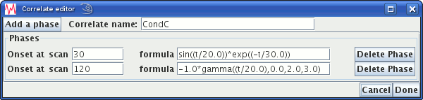
An function correlate design consists of a number (1 or more) functions from which the design matrix is calculated as the sum of all the functions. One function is specified per phase. Of course, you can simply have a singe phase which consists of all the functions you want to use added together, but you may find it simpler and easier to manage if you use a separate phase for each function.
You need to:
1. Give your correlate a name (in the "Correlate name" field), such as "CondC".
2. Add as many phases as you need to describe the correlate by clicking the button.
3. For each phase (function) set the time at which the function is defined to start (at which t=0 for the function). All functions evaluate to zero at times less than the time of onset. Depending on the setting or , the time variable (t) will be measured either in scan units or seconds.
4. For each phase, enter the function, using the independent variable t.
Above, we have set a correlate called "CondC" that uses two functions: the first is an exponentially-decaying sinusoid, and the second is an inverted gamma probability density function.
Click the button when you are finished, and a sketch of the design matrix will be shown in the General Linear Model tab for the correlate you just created.

For each correlate that you set, you will see a sketch of the design matrix next to the correlate name, as shown below for the three example correlates above.

design_matrix

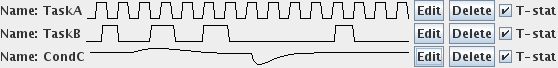
Note: these sketches are only to help you to be sure that you have created your correlates correctly; they are not correctly scaled vertically relative to one another.

Next to each correlate is the t_stat_check check-box. If selected, a T-static image for the corelate will be produced; if you do not want T-statistics for any particular correlate, then un-check this box.

Haemodynamic Response Function (HRF)

For functional MRI (fMRI) analysis you can use an HRF by selecting the use_hrf_check check-box. The design matrix you have set is convolved with the HRF to give the design matrix that is actually used in the GLM analysis. The HRF is defined using two gamma probability density functions, the standard parameters for which are similar to those used by SPM. However, you can change them by clicking on the edit_hrf_params_button button, which brings up the HRF editor dialog:

edit_hrf_params_dialog

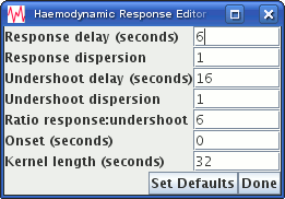
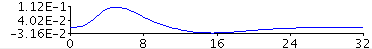
If you change any of the HRF parameters, the HRF shape shown plotted in the HRF display panel will be updated.

hrf_plot

Confounds

You use this tab to set 'confounding' basis function that are corrupting your data. You are not interested in these confounds, but you are interested in modelling them and removing them from your data.

dynamic_confounds

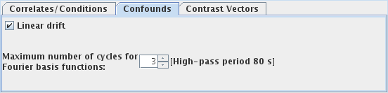
You can model and remove from you data:

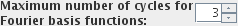A DC (constant-valued) offset. This is always performed, regardless of any settings here.
A linear 'drift' in your data by selecting .
Sinusoidal and co-sinusoidal oscillations in your data. You set the maximum number of oscillation cycles in your data using the spinner, and (as long as you have set the time between images and the number of time points correctly) Jim will calculate the equivalent high-pass filter period.

Note: you can have zero or more correlates. However, you must have fewer correlates and confounds (see below) than you have time points in your data. If you have no correlates, then only the confounds will be used in the GLM; you may wish to do this if you only want to remove confounds from your data, leaving just the residuals.

Contrast Vectors

The GLM analysis module will produce images showing the amplitudes of the correlates in the design matrix, and also will create T-statistic and p-value statistical parametric maps showing the significance of those correlates. However, you may also want to answer questions such as "what is the difference in activation between Task A and Task B". You can create statistics showing these in the "Contrast Vectors" tab:

glm_contrast_vectors

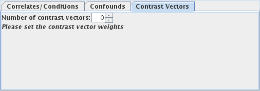
Select the number of contrast vectors you want to calculate, using the dynamic_n_contrasts_spinner spinner. This will create a set of weights for each contrast vector, whereby you can weight the correlate for each task. For example, imagine you wanted to look at the difference between "TaskA" and "TaskB", and also between "TaskB" and "CondC" in the example above.

contrasts

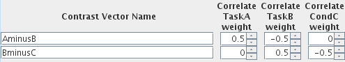
We have set the weights such that we will be looking at the differences between the correlates, and given these contrasts names to reflect those differences. You can use any names for the contrast vectors you wish.

When the GLM analysis is performed, additional SPMs will be produced (two for each contrast vector) - a T-statistic map and a p-value map. The names of the maps will be created using the names you set here.

Slice Order Correction and Bonferroni Correction

You can use this section to set additional processing settings:

glm_slice_order_correction

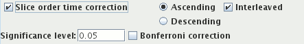
When you collect data for an MRI scan, the individual slices are normally acquired at different times. The order of slice collection may vary, starting with the first slice in the dataset, or the last slice, or the order may be interleaved (1,3,5,7, ...2,4,6,8, ...). You can correct for the slight time difference in the collection of the slices by selecting slice_order_check . Then set whether the slice order is:

if the first slice was collected first and the last slice was collected last (in time).
if the last slice was collected first and the first slice was collected last (in time).
if the slices were collected in the order 1,3,5,7, ... 2,4,6,8 ... (for ascending order), or N,N-2,N-4,N-6 ... N-1,N-3,N-5,N-7 (for descending order in an N-slice dataset).

The GLM module will produce T-statistic and p-value SPMs. You can set the significance level for these maps by altering the significance_level ; pixels where the statistic is below the significance level is zero will be given an T-value of zero or a p-value of 1.0 in the corresponding SPMs.

Because, for typical images, many thousands of statistical tests are being performed, it is likely that many pixels will show significance in the SPMs just by chance at a significance level of 0.05 (the default). However, you can perform a Bonferroni correction by selecting the bonferroni_correction check-box. The p-value is adjusted by taking the number set as the significance level and dividing it by the number of pixels that are tested using the GLM. Only those pixels that remain significant are output in the SPMs.

Residuals Image

Selecting the create_residuals_check

check-box will create output image(s) with the same names as the input image(s), but with the suffix "residuals". The residuals image(s) will be the result of subtracting the GLM from the input data. Residuals images can be useful for investigating whether fitting the GLM still leaves some "structure" - this would be the case if the GLM does not provide a compete description of the input images, and that possibly further correlates should be included in the model. In the case of a "complete" GLM, the residuals will consist entirely of Gaussian-distributed uncorrelated values.

Performing the Analysis

When you click the apply_button

button, the output images created will have names produced by taking the base name in the image output section and appending the suffixes from the correlate and contrast vector names you have provided. The p-value maps are also appended with "-p" and the T-statistic maps are appended with "-T".

When calculating statistical maps, the GLM analysis uses a two-pass analysis. The first fits the GLM to the data to produce a set of residuals that are, in general, auto-correlated. The auto-correlation is then estimated from the residuals, and a second pass corrects the p- and T-values for the auto-correlation in the data. Correction of the SPMs for auto-correlation follows the method of Woolrich et al..

Saving and Retrieving the GLM Specification

You can save the whole GLM setup, including the correlates, confounds, contrast vectors and haemodynamic response function to disk file in XML format by clicking on the save_glm_spec_button

button. This will bring up a File Chooser for you to select the XML file name.

Clicking on the load_glm_spec_button button will allow you to select an XML file where you previously save the setup, and reload it from disk.

The document type definition for a GLM specification file is given in the file formats section.

Jim Home